 相关文章:Math 4
The Last Straw: A Stopping-Time Problem Where e Shows Up Three Times
Draw random numbers uniformly from $[0,1]$, one at a time, and keep a running sum. Stop the moment the sum first exceeds 1. Let $X_N$ denote the last number drawn — the one that pushed the total over the edge, the proverbial last straw. The question:
$$
E[X_N] = \ ?
$$
At first glance this looks innocent. Every draw is $\mathrm{U}(0,1)$ with mean $\tfrac12$, so shouldn’t the answer be something boring like $\tfrac12$? It isn’t. The last draw is special: it was selected by the stopping rule, and that selection systematically favors larger numbers. Teasing out exactly how much larger takes us through one of the most elegant corners of elementary probability — and along the way, $e$ makes three separate appearances.
The answer, for the impatient:
$$
E[X_N] = \frac{4-e}{2} \approx 0.6409.
$$
Here is the full story.
Step 1: A Volume That Falls Out as $1/n!$
Write $S_n = X_1 + \cdots + X_n$. The event that the process is still running after $n$ draws is exactly ${S_n \le 1}$, so the whole problem hinges on understanding
$$
P(S_n \le 1).
$$
Think geometrically. The point $(X_1, \dots, X_n)$ is uniformly distributed over the $n$-dimensional unit cube $[0,1]^n$, and the region ${x_1 + \cdots + x_n \le 1}$ carves out a corner of that cube. Which corner? The simplex with vertices at the origin and the $n$ unit vectors.
- $n=1$: the interval $[0,1]$, length $1 = \tfrac{1}{1!}$. ✓
- $n=2$: the triangle under $x+y=1$, area $\tfrac{1}{2} = \tfrac{1}{2!}$. ✓
- $n=3$: the tetrahedron under $x+y+z=1$, volume $\tfrac{1}{6} = \tfrac{1}{3!}$. ✓
So we conjecture
$$
P(S_n \le 1) = \frac{1}{n!}.
$$
A trap worth flagging. In 2D, the line $x+y=1$ happens to pass through the center of the square $(\tfrac12, \tfrac12)$, so it cuts the square into two equal halves — the area $\tfrac12$ follows “for free.” The tempting generalization is that the plane $x+y+z=1$ bisects the cube. It does not! The plane passes through $(\tfrac13, \tfrac13, \tfrac13)$, not the cube center $(\tfrac12,\tfrac12,\tfrac12)$. The sliced-off piece is a tetrahedron with base area $\tfrac{\sqrt 3}{2}$ and height $\tfrac{1}{\sqrt 3}$, giving volume $\tfrac13 \cdot \tfrac{\sqrt3}{2}\cdot\tfrac{1}{\sqrt3} = \tfrac16$. The 2D bisection was a coincidence, and coincidences do not generalize.
One refinement we will need later: for $0 \le s \le 1$, scaling the simplex by $s$ gives
$$
P(S_n \le s) = \frac{s^n}{n!}.
$$
Step 2: $E[N] = e$, the First Appearance
The event ${N > n}$ — “still running after $n$ draws” — is precisely ${S_n \le 1}$. So the tail probabilities of the stopping time are exactly the volumes we just computed:
$$
P(N > n) = \frac{1}{n!}.
$$
For a nonnegative integer-valued random variable, $E[N] = \sum_{n \ge 0} P(N > n)$. Hence
$$
E[N] = \frac{1}{0!} + \frac{1}{1!} + \frac{1}{2!} + \frac{1}{3!} + \cdots = e.
$$
(Note the two leading ones — the $n=0$ and $n=1$ terms are both $1$. Dropping one of them and concluding $E[N] = e-1$ is a classic slip.) On average, it takes $e \approx 2.718$ draws to push the sum past 1. There is $e$, for the first time.
Step 3: The Last Draw Is Not Uniform — the Key Insight
Now the heart of the problem. Condition on the state of the sum just before the final draw: suppose $S_{N-1} = s$ (note $s \le 1$, since the process was still alive). The last draw $X_N$ started life as an ordinary $\mathrm{U}(0,1)$ random variable, but it was filtered by a condition: it must satisfy $X_N > 1 - s$.
A uniform random variable, conditioned to exceed a threshold, is still uniform — just on a truncated range:
$$
X_N \mid S_{N-1} = s \ \sim\ \mathrm{U}(1-s,\ 1)
\quad\Longrightarrow\quad
E[X_N \mid S_{N-1} = s] = 1 - \frac{s}{2}.
$$
This is the size-bias effect: the last straw is pushed upward because only straws large enough to cross the line get to be the last straw. Averaging over the random threshold via the law of total expectation,
$$
E[X_N] = 1 - \frac{1}{2},E[S_{N-1}],
$$
and the problem reduces to computing $E[S_{N-1}]$ — the expected sum just before stopping.
Two sanity checks kill the tempting shortcuts here. Substituting $E[N] = e$ for $E[S_{N-1}]$ yields $1 - \tfrac{e}{2} < 0$ — impossible for a positive random variable. Even the fix $(E[N]-1)\cdot\tfrac12 = \tfrac{e-1}{2} \approx 0.86$ fails, because the draws that survive (don’t trigger a stop) are biased toward small values. The truth is smaller, and we now compute it exactly.
Step 4: $E[S_{N-1}] = e - 2$, the Hard Part
The indicator decomposition
The pre-stopping sum collects $X_i$ exactly when the process is still alive after the $i$-th draw:
$$
S_{N-1} = \sum_{i=1}^{\infty} X_i \cdot \mathbf{1}{S_i \le 1}
\quad\Longrightarrow\quad
E[S_{N-1}] = \sum_{i=1}^{\infty} E\big[X_i \cdot \mathbf{1}{S_i \le 1}\big].
$$
Another trap: $E[XY] \ne E[X]E[Y]$
The seductive move is to split the expectation: $E[X_i]\cdot P(S_i \le 1) = \tfrac12 \cdot \tfrac{1}{i!}$. But $X_i$ and the survival indicator $\mathbf 1{S_i \le 1}$ are negatively correlated — a larger $X_i$ makes survival harder. Splitting overestimates.
Check it brutally for $i=2$ by integrating directly over the familiar triangle:
$$
E\big[X_2 \cdot \mathbf 1{X_1 + X_2 \le 1}\big]
= \int_0^1 \int_0^{1-x} y ,\mathrm{d}y,\mathrm{d}x
= \int_0^1 \frac{(1-x)^2}{2},\mathrm{d}x
= \frac{1}{6}.
$$
The split version gives $\tfrac12 \cdot \tfrac12 = \tfrac14$ — an overestimate by 50%. There is no way around the correlation; we need the conditional expectation.
Symmetry to the rescue
Conditioned on landing in the simplex ${x_1 + \cdots + x_i \le 1}$, the point $(X_1,\dots,X_i)$ is uniform, and all $i$ coordinates play symmetric roles. For a uniform distribution over a convex region, the expected position is the centroid, and the centroid of this simplex is
$$
\Big(\frac{1}{i+1}, \dots, \frac{1}{i+1}\Big)
\quad\Longrightarrow\quad
E[X_i \mid S_i \le 1] = \frac{1}{i+1}.
$$
(Why centroid = expectation? A uniform density is a constant $1/V$, so $E[\text{coordinate}] = \frac{1}{V}\int x ,\mathrm{d}x$ — literally the definition of the centroid. This shortcut is a privilege of uniformity; for a Gaussian you must integrate honestly.)
Multiplying the conditional mean by the survival probability:
$$
E\big[X_i \cdot \mathbf{1}{S_i \le 1}\big]
= \frac{1}{i+1}\cdot\frac{1}{i!}
= \frac{1}{(i+1)!}.
$$
The $i=2$ check: $\tfrac13 \cdot \tfrac12 = \tfrac16$. ✓ — matching the brute-force integral.
Summing up
$$
E[S_{N-1}] = \sum_{i=1}^{\infty} \frac{1}{(i+1)!}
= \sum_{j=2}^{\infty} \frac{1}{j!}
= e - 2 \approx 0.7183.
$$
There is $e$ again.
Step 5: Assembly
$$
E[X_N] = 1 - \frac{E[S_{N-1}]}{2} = 1 - \frac{e-2}{2} = \frac{4-e}{2} \approx 0.6409.
$$
And $e$ appears a third time, hiding inside the answer. As a bonus consistency check, the expected total sum at stopping is
$$
E[S_N] = E[S_{N-1}] + E[X_N] = (e-2) + \frac{4-e}{2} = \frac{e}{2} \approx 1.359.
$$
Monte Carlo Verification
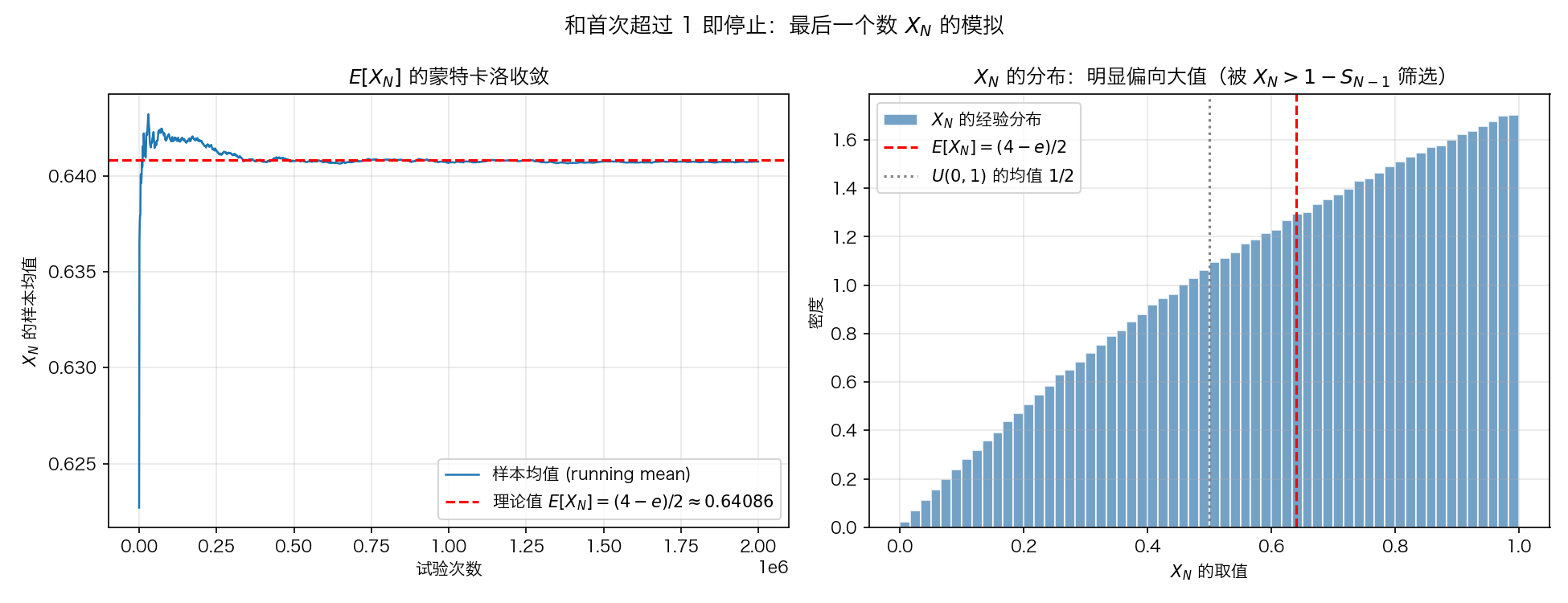
Two million simulated runs confirm everything (simulation script: a dozen lines of Python):
| Quantity | Simulated | Theory | Error |
|---|---|---|---|
| $E[N]$ | 2.71902 | $e$ | 0.00074 |
| $E[S_{N-1}]$ | 0.71859 | $e-2$ | 0.00030 |
| $E[X_N]$ | 0.64076 | $\tfrac{4-e}{2}$ | 0.00010 |
| $E[S_N]$ | 1.35935 | $\tfrac{e}{2}$ | 0.00021 |
Left: the running mean of $X_N$ converging to the theoretical value. Right: the empirical distribution of $X_N$ — density increasing with $x$, nearly vanishing near zero.
| |
The empirical distribution of $X_N$ is also worth a look: its density increases with $x$, nearly vanishing near zero. The last straw is almost never a small number — the size-bias of Step 3, visible in the raw histogram.
Takeaways
Three traps, three lessons:
- A count is not a sum. $E[N] = e$ counts draws; $S_{N-1} \le 1$ bounds a sum. Mixing them produced a negative expectation — the sanity check caught it instantly.
- Expectation of a product is not the product of expectations, unless the factors are independent. Here the correlation is structural (survival selects small values), and ignoring it cost 50%.
- Coincidences do not generalize. The 2D bisection $P(S_2 \le 1) = \tfrac12$ held only because $x+y=1$ passes through the square’s center. The 3D analogue fails. Always ask why a pattern held before extending it.
And one positive lesson: when a uniform distribution is conditioned on a region, its expectation is the region’s centroid. Geometry can replace a page of integration.
Further Exploration
What if the threshold moves to 2? The skeleton of the argument survives — the crux is still $P(S_n \le s)$ — but for $s > 1$ the plane no longer cuts a clean corner off the cube: the simplex gets truncated by the cube’s far faces, and inclusion–exclusion enters the game. That variant is left as an exercise, with the honest warning that it is substantially messier than this one.